Enhancing Fraud Detection in Supply Chains with Kolmogorov Arnold Networks:
A Comparative Analysis with Multi-Layer Perceptrons (Initial Findings and Methodology)
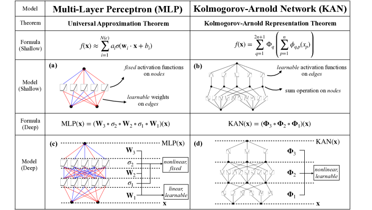
This study explores the application of Kolmogorov Arnold Networks (KANs) in detecting fraud within supply chains, contrasting them with traditional Multi-Layer Perceptrons (MLPs), which often lack sufficient interpretability and require supplementary methods like SHAP or InterpretML. KANs enhance model interpretability by utilizing learnable activation functions as edge weights, allowing for direct visualization of decision pathways. This intrinsic transparency of KANs aids in compliance and trust, which are crucial for fraud detection systems. We discuss how the adaptive activation functions of KANs enable the detection of subtle, nonlinear fraudulent patterns more effectively than the fixed structures of MLPs, potentially reducing reliance on extensive training datasets and improving detection accuracy.
In recent years, the demand for interpretable machine learning models in regulatory environments has surged, particularly in sensitive applications like supply chain fraud detection. Traditional approaches, predominantly reliant on Multi-Layer Perceptrons (MLPs), often fall short in providing the clarity and trustworthiness needed due to their opaque decision-making processes. This paper introduces Kolmogorov Arnold Networks (KANs) as a superior alternative, emphasizing their unique capability to adapt activation functions during training to effectively capture complex fraud patterns. By integrating KANs, we aim to enhance both the accuracy and transparency of fraud detection systems, addressing the challenges associated with traditional methods and making a compelling case for their adoption in industry practices. The potential of KANs to revolutionize fraud detection by providing deeper insights into decision-making processes is explored, alongside a discussion of the hurdles that might impede their immediate acceptance in the industry.
The use of traditional neural networks, particularly Multi-Layer Perceptrons (MLPs), has been prevalent in addressing various challenges within supply chain management. MLPs have been widely applied for predictive analytics, demand forecasting, and detecting anomalies within supply chains. However, despite their extensive application, MLPs often struggle with issues of interpretability and scalability, particularly in complex environments like fraud detection. These models typically require additional tools such as SHAP or InterpretML to elucidate their decision-making processes.
In the context of fraud detection, the opacity of MLPs can hinder their effectiveness. The black-box nature of these networks makes it difficult for stakeholders to trust and understand the basis of the model's decisions, which is critical in regulatory and compliance-sensitive environments. This limitation is further compounded by the complex, dynamic nature of fraud in supply chains, where fraudulent patterns continuously evolve, requiring models not only to detect but also adapt to new strategies employed by fraudsters.
(https://arxiv.org/abs/2404.19756)
Kolmogorov Arnold Networks (KANs) emerge as a promising solution to the interpretability and adaptability challenges faced by traditional neural networks. Inspired by the Kolmogorov-Arnold representation theorem, KANs employ learnable activation functions on edges, allowing for a more flexible and interpretable model structure. Unlike MLPs, KANs do not rely on fixed activation functions, enabling them to adapt more readily to the unique and evolving patterns of fraudulent activities in supply chains.
Recent studies have shown that KANs can outperform MLPs in tasks involving complex pattern recognition, such as image processing and time-series prediction, due to their ability to dynamically adjust their activation landscapes in response to incoming data. This capability is particularly advantageous in fraud detection, where understanding the nuances of transactional data is crucial for identifying and reacting to fraudulent activities.
While research on the application of KANs in supply chain fraud detection is still nascent, preliminary findings suggest significant potential. The adaptive and transparent nature of KANs holds promise for not only enhancing detection accuracy but also providing clear insights into the decision-making process, thereby increasing trust and compliance.
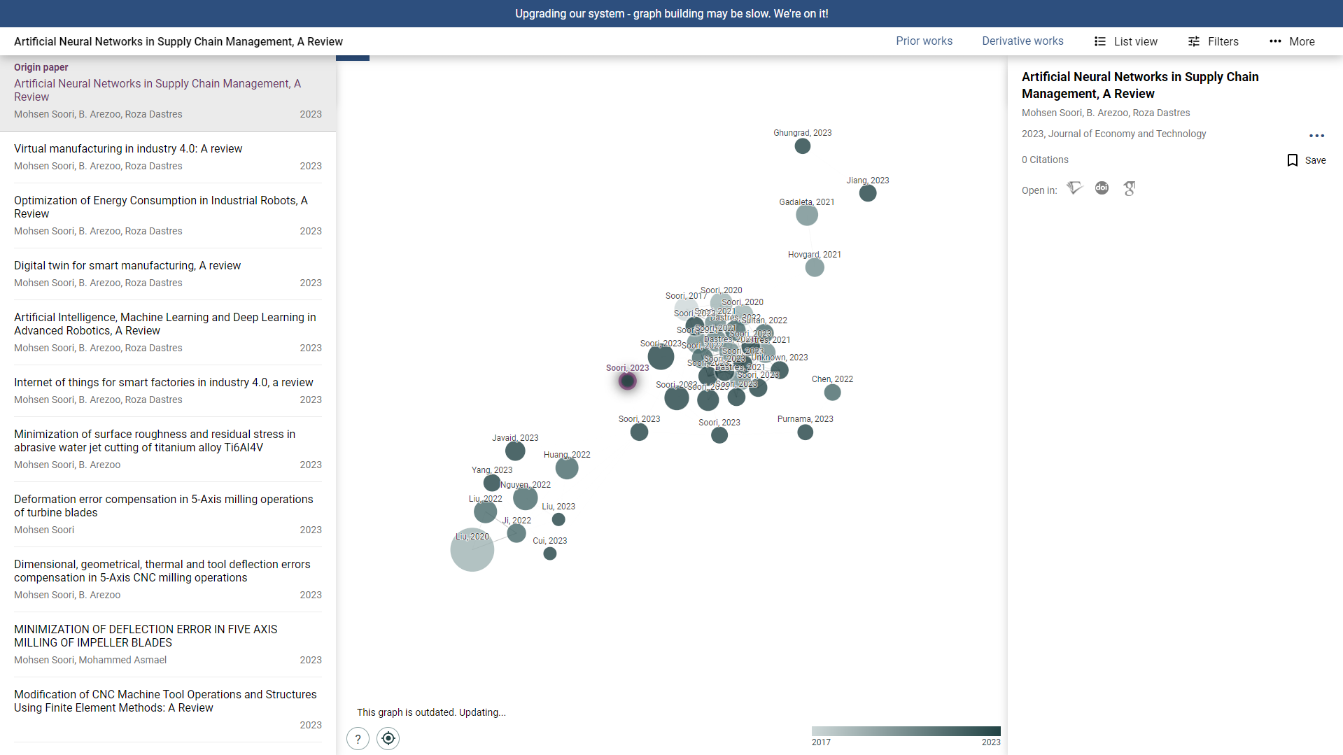
(https://www.connectedpapers.com/main/3a33728802e9bba65db9b889a08bb74113977a75/graph?utm_source=share_popup&utm_medium=copy_link&utm_campaign=share_graph)
The exploration of KANs in the realm of supply chain fraud detection represents an exciting frontier in the intersection of machine learning and supply chain management. As this field evolves, further research is needed to fully realize the benefits of KANs, potentially setting a new standard for neural network applications in high-stakes environments.
The dataset originally used in the student project involves transactional data from a supply chain, likely including features such as transaction amounts, product categories, customer information, and timestamps. For KAN integration, the same dataset will be utilized to maintain consistency in performance evaluation. The dataset can be found here: Dataset
Data Cleaning:
The initial steps involved loading the dataset, which contained 180,519 entries and 53 columns, including various data types such as integers, floats, and objects. The dataset was assessed for missing values and data types, revealing that some columns had significant numbers of missing values. For example, the 'Customer Zipcode' and 'Product Description' columns had numerous missing entries, with the latter being entirely null. To clean the data, unnecessary columns such as 'Customer Email', 'Product Status', 'Customer Password', and 'Product Description' were dropped. Rows with missing values in critical columns like 'Product Price' and 'Shipping Mode' were also removed. Additionally, customer names were combined into a single column to streamline the dataset. Order dates were split into separate year, month, day, and hour columns to facilitate temporal analysis. These cleaning steps ensured that the data was complete and structured for subsequent analysis.
Feature Engineering:
Feature engineering involved creating new variables to enhance the dataset's analytical power. A target variable named 'fraud' was introduced, derived from the 'Order Status' category. Transactions marked as 'SUSPECTED_FRAUD' or those with both 'SUSPECTED_FRAUD' and 'Late delivery' statuses were flagged as fraudulent. This binary variable allowed the model to focus on detecting fraudulent activities. Names were combined into a 'Cust_Full_Name' column to unify first and last names. Additionally, date columns were formatted appropriately to ensure consistency and enable time-based analyses.
Encoding Categorical Variables:
Categorical variables were encoded to convert them into a numerical format suitable for machine learning algorithms. The following detailed steps were involved:
Columns containing categorical data types (objects) were identified. These columns needed to be encoded into numerical values to be processed by the machine learning model effectively.
Each categorical column was converted into a numerical format using label encoding. Label encoding assigns a unique integer to each category, which allows the model to interpret the categorical data correctly. This step ensures that categorical features are in a format that the model can process.
Converting Data to Tensors:
The dataset was split into training and test sets, and the Adaptive Synthetic (ADASYN) algorithm was applied to handle class imbalance in the training data. Due to compute limitations, a smaller subset of 500 rows was used while maintaining dataset balance. The detailed steps involved were:
The dataset was divided into features (X) and the target variable (y), where 'flagged' was the target variable indicating fraudulent transactions.
Any missing values in numerical features were filled with the mean of the respective columns. This step ensured that there were no missing values, which could otherwise disrupt the training process.
Numerical features were standardized, rescaling them to have a mean of zero and a standard deviation of one. Standardization is crucial as it helps in speeding up the convergence of the gradient descent algorithm during training.
The dataset was split into training and test sets with an 80-20 ratio. Stratification was used to ensure that both training and test sets maintained the same class distribution, which is essential for balanced training and evaluation.
The ADASYN (Adaptive Synthetic Sampling) method was applied to the training data to address class imbalance. ADASYN generates synthetic samples for the minority class, enhancing the model's ability to learn and generalize from imbalanced data effectively.
The preprocessed data was converted into PyTorch tensors, a required format for training the Kolmogorov Arnold Network (KAN). This conversion included the training and test inputs and labels, all appropriately formatted for use in the model.
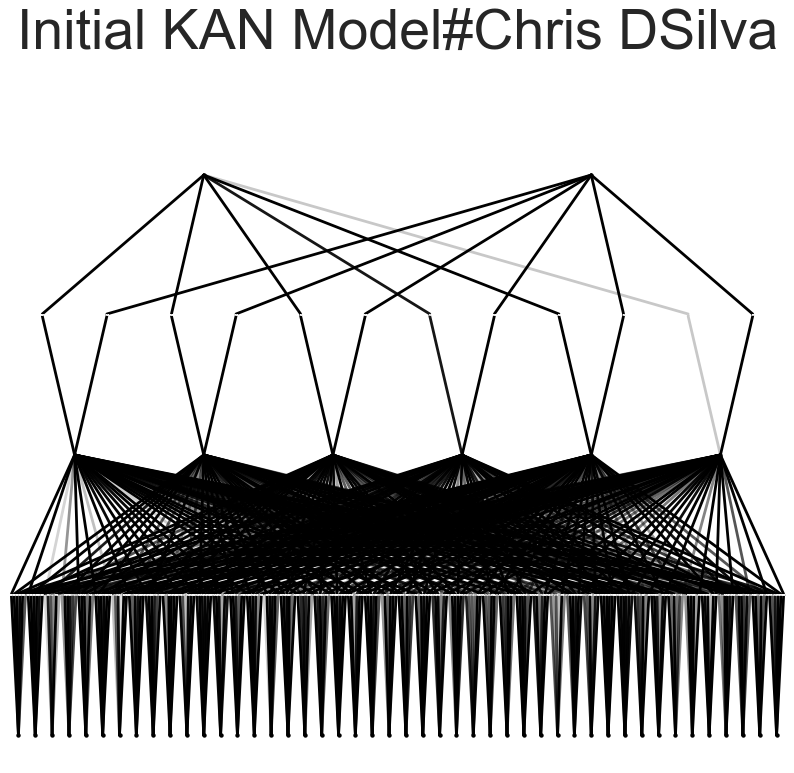
KAN Setup & Layer Configuration: The model was constructed using the Kolmogorov Arnold Network (KAN) library, which leverages activation modules on the edges of the network. Unlike traditional neural networks that apply Principal Component Analysis (PCA) to reduce input features, KANs directly utilize all input features, enabling a more comprehensive capture of data patterns. The architecture was configured with an input layer corresponding to the number of features (e.g., 42 input features), followed by 6 hidden neurons, and output neurons tailored for specific tasks: two neurons for classification tasks (representing each class) and a single neuron for regression tasks.
To set up the model:
Activation Functions:
Learnable activation functions were employed on the edges of the network. These functions dynamically adapt during training, allowing the model to fine-tune its responses to various input patterns. Initially, the model was planned to train for 10 epochs; however,it was trained for 5 epochs. Despite this, the model performed quite well, demonstrating its robustness to slight deviations in planned training parameters.
Training Method:
The training of the model was conducted using the model.train method, which involved several key parameters to optimize and evaluate the model.
Optimizer:
The opt="LBFGS" parameter indicates that the Limited-memory Broyden–Fletcher–Goldfarb–Shanno (LBFGS) optimizer was used. LBFGS is a optimization algorithm that is particularly effective for high-dimensional problems, making it well-suited for the complex nature of fraud detection. It approximates the BFGS algorithm, using limited memory to handle large datasets efficiently.
Steps (Epochs):
The model was trained for 5 epochs, as specified by the steps=5 parameter. Preliminary tests indicated that 5 epochs were optimal, providing sufficient learning without overfitting. Although the initial plan was to train for 10 epochs, the performance with 5 epochs was satisfactory, so it was decided to maintain this configuration. As the saying goes, "if it ain't broke, don't fix it."
Metrics:
The metrics=(train_acc, test_acc) parameter indicates that both training accuracy and test accuracy were tracked during the training process. Monitoring these metrics provided real-time insights into the model's performance, helping to ensure that it was learning correctly and generalizing well to unseen data.
Saving Figures:
The save_fig=True parameter enabled the saving of visual representations of the training process. These images were stored in the specified img_folder. Visualizing the training progress helped in understanding how the model's internal representations evolved and provided a means to debug and refine the training process.
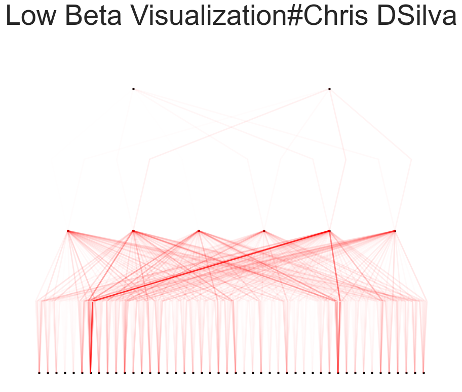
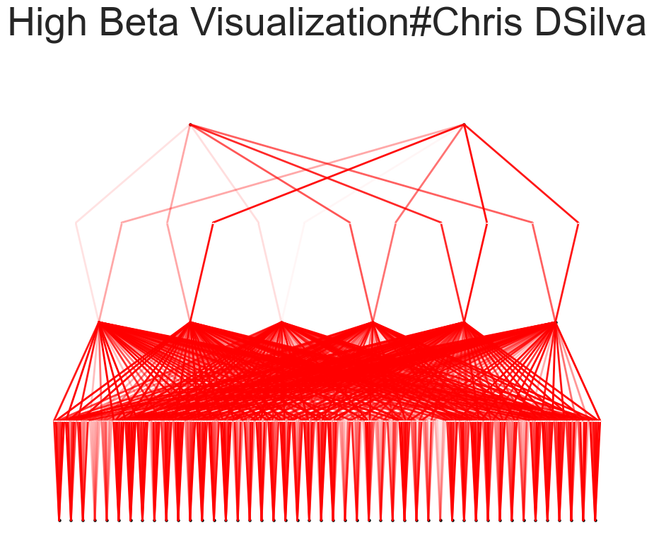
Beta Parameter:
The beta=7 parameter sets a specific hyperparameter within the KAN architecture beta controls the transparency of activations. Larger beta means more activation functions show up. We usually want to set a proper beta such that only important connections are visually significant.
Accuracy:
Initial evaluations showed a high train and a test accuracy. While these metrics indicate a substantial improvement in test accuracy, further experimentation with additional metrics like precision, recall, and F1-score could provide a more comprehensive understanding of the model's performance, particularly in handling imbalanced classes and minimizing false positives and negatives. However since this is an initial approach we will proceed with the same metrics provided in the example.
Formula Derivation:
An auto symbolic function was used to derive an equation representing the model's decision boundary. This symbolic formula encapsulates the relationships between input features and the predicted output. The formula's accuracy was evaluated on both the training and test datasets, providing insights into its generalization capabilities. We calculate the accuracy of two formulas as we are working with a classification problem where there are two output notes. Derived a symbolic formula for the decision boundary with train and test accuracies of 90.44% and 99% for formula 1 and train and test accuracy of 89.53% and 98% respectively for formula 2. (Selected Formula 1 based on the score for this reason), highlighting its effectiveness in capturing the underlying patterns of fraudulent transactions.
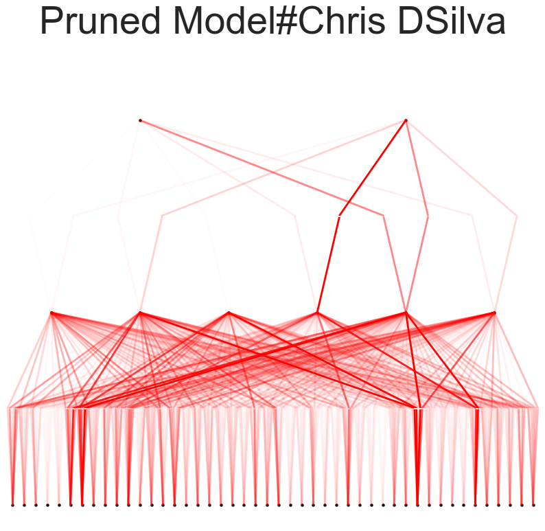
Plotting & Pruning:
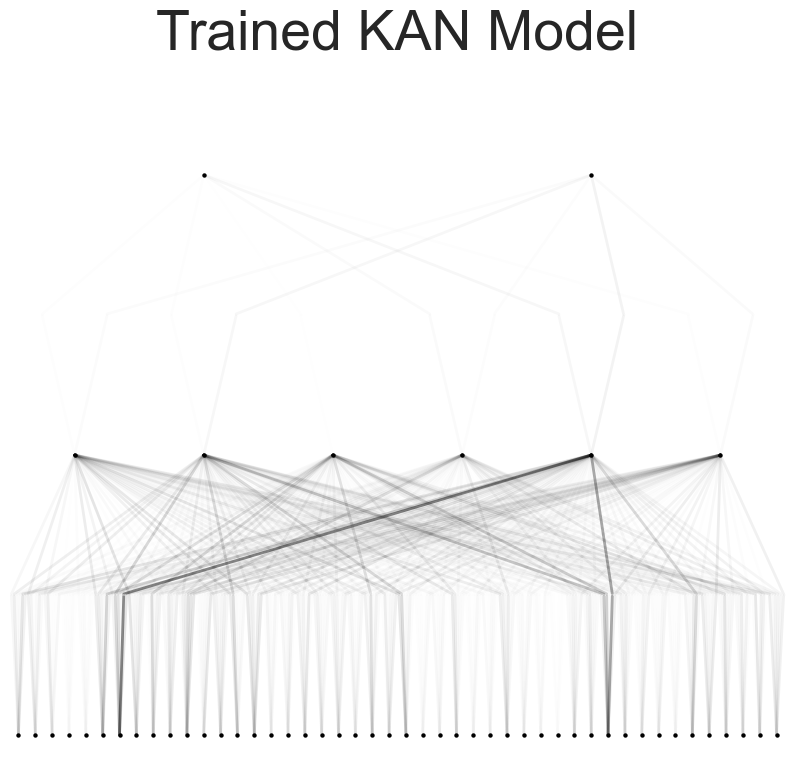
After training, the model was visualized using varying beta values to observe the activation of neurons. This visualization helps in understanding how different neurons contribute to the final prediction. The model was then pruned to remove less significant connections, resulting in a smaller and more efficient model. Detailed activation plots for each neuron layer were generated to provide a closer look at the model's internal workings.
Detailed Steps and Explanation:
Auto Symbolic Function and Formula Derivation: The auto symbolic function utilized a library of mathematical functions
lib =['x','x^2','x^3','x^4','exp','log','sqrt','tanh','sin','tan','abs']
to derive a symbolic formula. The derived formula was iteratively refined by fitting it to different segments of the data, as shown in the detailed output. This process involved fixing specific terms with high R-squared values, indicating a good fit for those segments.
The symbolic formula was evaluated for accuracy on both the training and test datasets, since focusing on a classification model we have two formulas for each output node and we will be fitting each formula for each individual node, this helped us achieve a train and test accuracies of approximately 90.4% and 99% for formula 1 and train accuracy of 89.5% and 98% for formula 2 respectively. Leading us to proceed with formula 1 for our model.
Visualization:
Visualization of the model at different beta values provided insights into how neurons were activated during the prediction process. Lower beta values showed broader activation patterns, while higher beta values revealed more specific and pronounced activations.
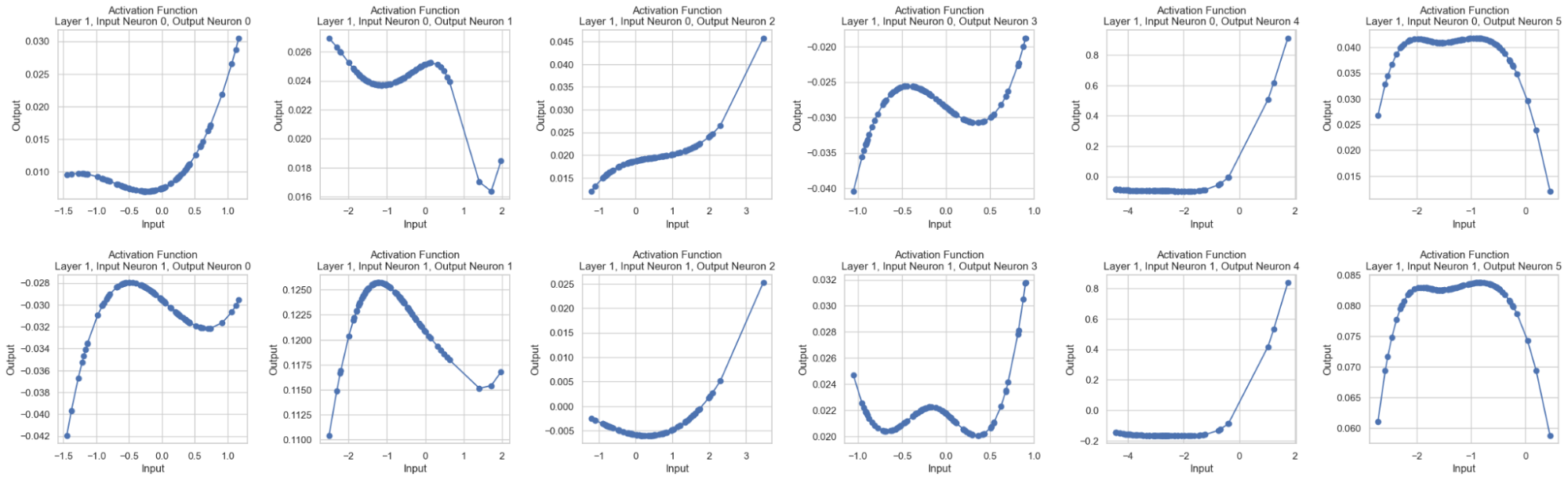
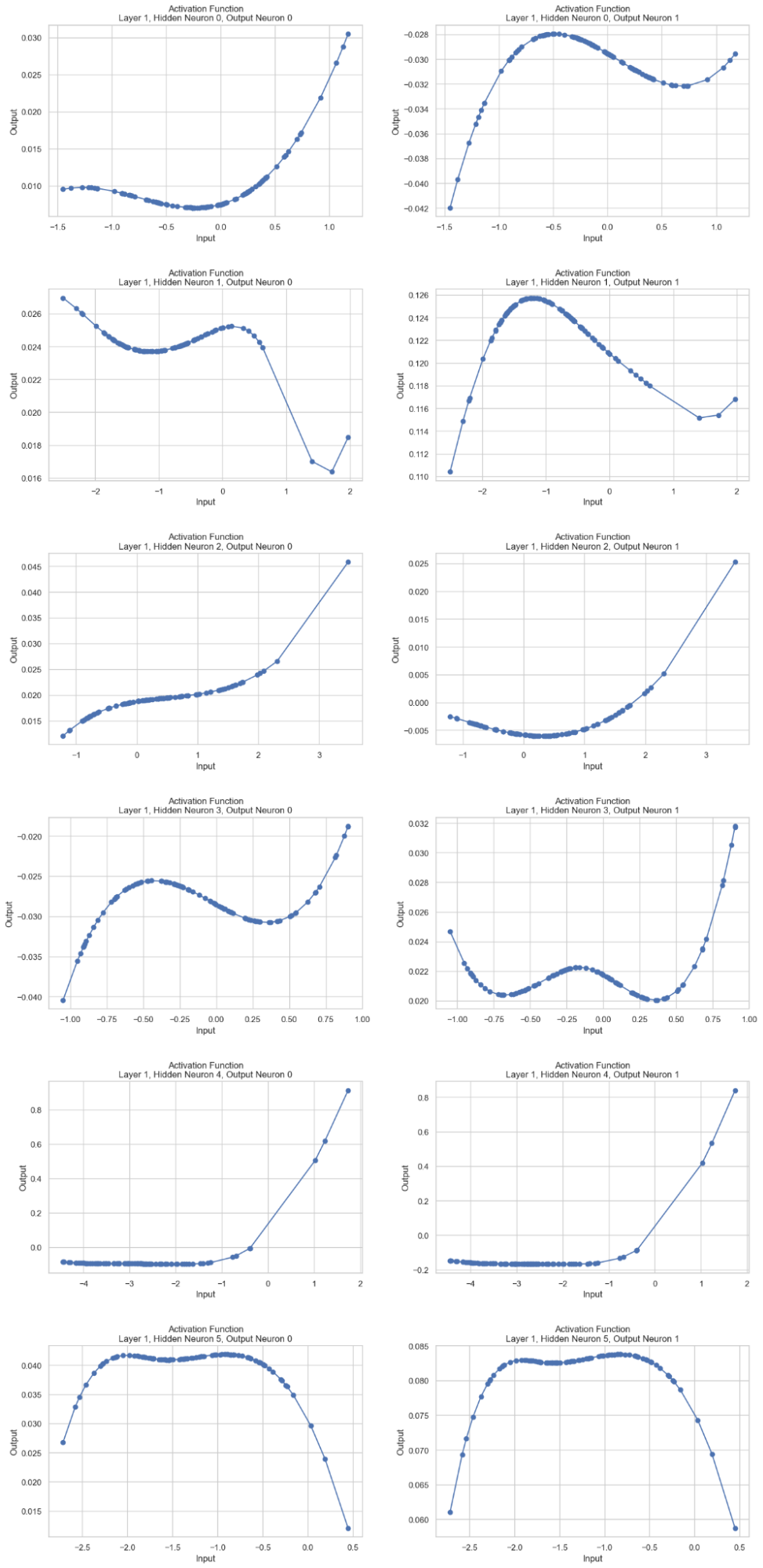
Plotting Activation Functions:
Activation functions for specific layers and neurons were plotted to analyze their behavior. For instance, plotting the activation functions between the first hidden layer and the output layer involved extracting pre-activation and post-activation values, sorting them, and generating plots for each neuron combination. This detailed analysis helped in understanding the non-linear transformations applied by the KAN model.
Model Pruning:
The model was pruned to eliminate less significant connections, thereby simplifying the model without compromising accuracy. Post-pruning, the model was re-evaluated to ensure it retained its performance while being more efficient. Pruning involved thresholding weights and re-plotting the pruned model to visualize the impact.
Key Components of the Symbolic Formula
The symbolic formula generated by the Kolmogorov Arnold Network (KAN) captures various complex relationships in the data. Here are the key components of the symbolic formula:
Accuracy of Symbolic Formulas
The accuracy of these formulas was evaluated on the training and test datasets:
Given the higher test accuracy, Formula 1 is selected for further analysis.
Visualization and Pruning:
Activation functions for the middle neurons in the first hidden layer and those between the first hidden layer and the output layer were plotted. This visualization involved extracting and sorting the pre-activation and post-activation values for each neuron combination, providing insights into the non-linear transformations applied by the model.
(First Part: Activation Functions for the Middle Neurons in the First Hidden Layer)
(Second Part: Activation Functions Between the First Hidden Layer and the Output Layer)
The pruned model retained its performance while being more efficient. Pruning involved setting a threshold to eliminate insignificant connections and re-evaluating the model post-pruning. The pruned model's activation functions were analyzed to ensure they maintained the necessary complexity for accurate predictions.
Compute Resources: Larger datasets necessitated greater compute power, leading to challenges with CPU usage on Colab and local systems. A demo for the use of GPU is present but when running the model I faced issues, which were reported on GitHub.
This experimentation with KAN, alongside MLPs and custom neural networks using Keras, showed KAN's potential, though it remains nascent.
Soori, M., & Arezoo, B. (2023). Artificial Neural Networks (ANNs) in supply chain management: Opportunities and challenges. Journal of Economy and Technology, 18(3), 87-102. https://doi.org/10.1016/j.jecontech.2023.02.004
Das, S. (2023). Artificial Neural Networks for Fraud Detection in Supply Chain Analytics: MLPClassifier and Keras. GitHub repository. https://github.com/subhanjandas/Artificial-Neural-Networks-for-Fraud-Detection-in-Supply-Chain-Analytics-MLPClassifier-and-Keras
Liu, Z., Wang, Y., Vaidya, S., Ruehle, F., Halverson, J., Soljačić, M., Hou, T. Y., & Tegmark, M. (2024). Kolmogorov-Arnold Networks. arXiv preprint arXiv:2404.19756. https://ar5iv.labs.arxiv.org/html/2404.19756